22 R: ggplot2
-
R package
ggplot2provides comprehensive options for plotting -
The package is developed with the philosophy of grammar of graphics
-
Here, we provide some minimal examples of creating plots using ggplot2
22.1 ggplot2: Overview
Grammar of Graphics: ggplot2 by Hadley Wickham
Install
ggplot2in your current R environment:install.packages('ggplot2')From RStudio:
Tools > Install Packagesand selectggplot2in the package name text boxThe initial gg in
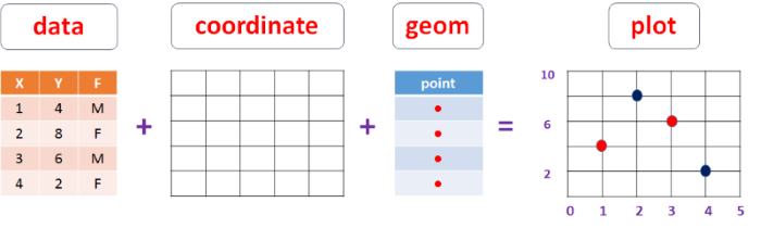
ggplot2stands for grammar of graphics based on the concept the grammar of graphics by Leland Wilkinson.Grammar of Graphics: The grammar tells us that a statistical graphic is a mapping from data to aesthetic attributes (colour, shape, size) of geometric objects (points, lines, bars). The plot may also contain statistical transformations of the data and is drawn on a specific coordinates system.
22.2 Steps of ggplot
Start with
ggplot()Supply a dataset
Include aesthetic mapping with
aes()Add layers as needed
Add on geom objects
geom_point()orgeom_histogram()Add scales like
scale_colour_brewer()Add faceting specifications like
facet_wrap()Add coordinate systems (like
coord_flip()
22.3 Essential part 
| Arguments | Explanation |
|---|---|
| data = | The DATA that you want to plot |
| aes() | AESTHETICS of the geometric and statistical objects, such as color, size, shape and position. |
| geom_ | The GEOMETRIC shapes that will represent the data. |
22.4 Advanced part
| Arguments | Explanation |
|---|---|
| stat_ | STATISTICAL summaries of the data that can be plotted, such as quantiles, fitted curves (loess, linear models, etc.), sums and so o. |
| coord_ | The transformation used for mapping data COORDINATES into the plane of the data rectangle. |
| facet_ | The arrangement of the data into a grid of plots |
| theme_ | The overall visual THEMES of a plot: background, grids, axe, default typeface, sizes, colors, etc. |
| scale_ | MAP between the data and the aesthetic dimensions, such as data range to plot width or factor values to colors. |
22.5 Geometric functions
| Function | Plot | Graphical_parameters |
|---|---|---|
geom_histogram |
Histogram |
colour, fill, alpha
|
geom_freqpoly |
Frequency polygon |
colour, fill, alpha
|
geom_density |
Density plot |
colour, fill, alpha, linetype
|
geom_rug |
Rug plot |
colour, side
|
geom_qq |
Quantile-Quantile plot |
colour, alpha, linetype, size
|
geom_boxplot |
Box plot |
colour, fill, alpha, notch, width
|
geom_violin |
Violin plot |
colour, fill, alpha, linetype, size
|
geom_point |
Scatter plot |
colour, alpha, shape, size
|
geom_jitter |
Jittered points |
colour, alpha, shape, size
|
geom_text |
Text |
colour, alpha, size, label, family, fontface
|
geom_bar |
Bar chart |
colour, fill, alpha
|
geom_line |
Line graph |
colour, alpha, linetype, size
|
geom_hline |
Horizontal line |
colour, alpha, linetype, size
|
geom_vline |
Vertical line |
colour, alpha, linetype, size
|
geom_smooth |
Fitted line |
method, formula, colour, fill, linetype, size
|
22.6 Read Data
Load ggplot2 library in the R environment
Set the working directory to the data folder and read the iris dataset as an R object DF.
DF = read.csv('iris.csv')
22.7 Single variable
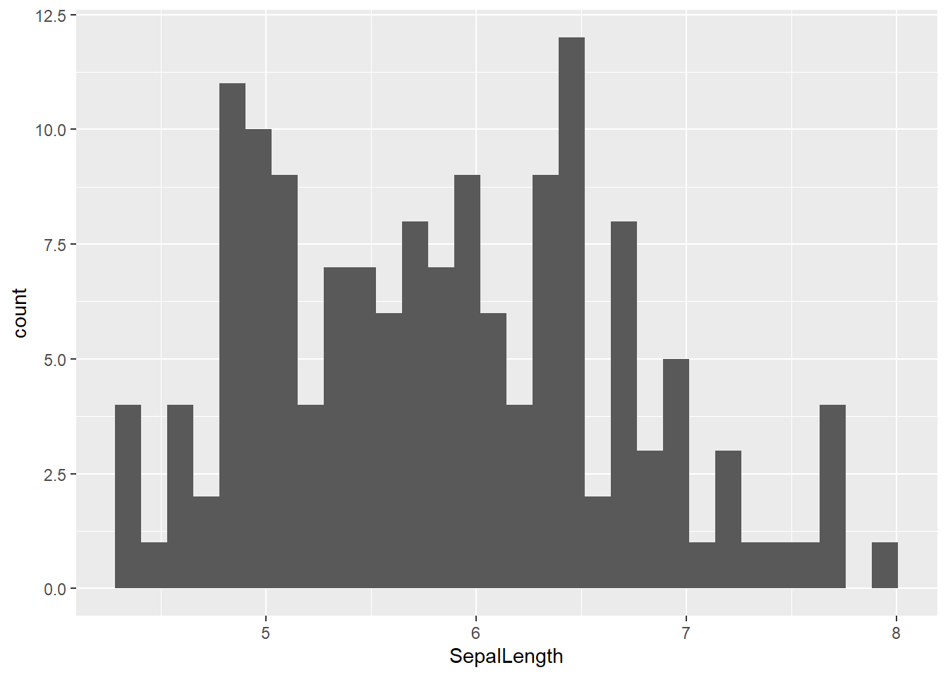
22.7.2 Density plot
g = ggplot(data = DF, mapping = aes(SepalLength)) + geom_histogram(aes(y = ..density..))
g = g + geom_density()
g
22.8 Multple variables
22.8.1 Scatter plot
g = ggplot(data = DF, mapping = aes(x = SepalLength, y = PetalLength)) + geom_point()
g
22.8.2 Scatter plot with group
g = ggplot(data = DF, mapping = aes(x = SepalLength, y = PetalLength, color = Species)) + geom_point()
g
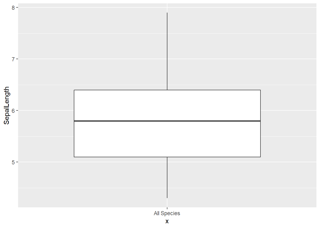
22.8.4 Boxplot
g = ggplot(data = DF, mapping = aes(x = Species, y = SepalLength)) + geom_boxplot()
g
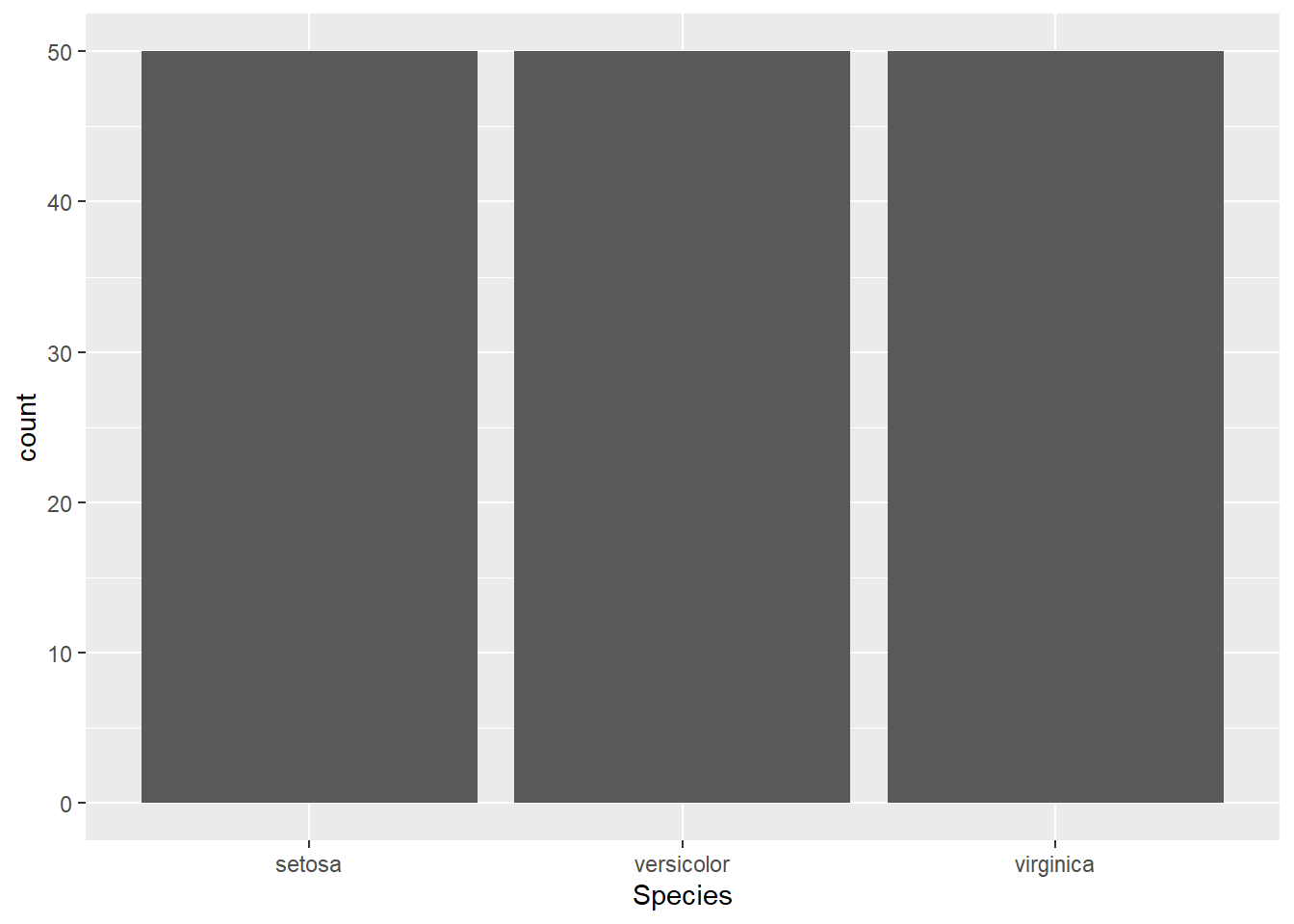
g = ggplot(data = DF, mapping = aes(x = Species, y = SepalLength, colour = Species))
g = g + geom_boxplot() + facet_wrap( ~ Species)
g