Section 31 Linear Regression Model: Prediction
31.1 Prediction from the model
\[ \large fm \leftarrow lm(SBP \sim BMI, \space data=BP) \]
\[ \large predict(fm, \space newdata=X, \space se.fit=TRUE, \space interval=`confidence`) \]
Call:
lm(formula = SBP ~ BMI, data = BP)

Residuals:
    Min      1Q  Median      3Q     Max
-8.3636 -2.1681  0.1586  2.1492  6.5777

Coefficients:
            Estimate Std. Error t value Pr(>|t|)
(Intercept) 36.20368    1.48011   24.46   <2e-16 ***
BMI          2.63229    0.05903   44.59   <2e-16 ***
---
Signif. codes:  0 '***' 0.001 '**' 0.01 '*' 0.05 '.' 0.1 ' ' 1

Residual standard error: 2.756 on 498 degrees of freedom
Multiple R-squared:  0.7997,    Adjusted R-squared:  0.7993
F-statistic:  1989 on 1 and 498 DF,  p-value: < 2.2e-16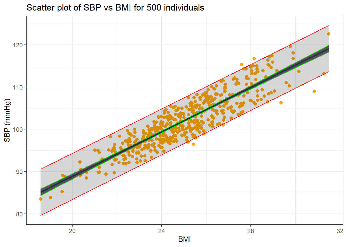
31.2 Explanation
Statistical Model
\[ \large y_{i} = \beta_0 + \beta_1 x_{i} + \epsilon_{i} \]
Prediction
\[ \large E(y|X=x^*) = \hat y^* = \hat \beta_0 + \hat \beta_1 x^* \]
Confidence Intervals for the mean value of y (population regression line)
\[ \large Var(\hat y^*) = \hat\sigma^2 \left[ \frac{1}{n} + \frac{(x^* -\bar x)^2}{S_{xx}} \right] \]
\[ \large SE(\hat y^*) = \sqrt {Var(\hat y^*)} \]
\[ \large CI_{0.95}(\hat y^*) = \left[ \hat y^* \pm t_{0.025, df_{residual}} * SE(\hat y^*) \right]\]
Prediction Intervals for the single value of y, i.e. actual value of y
The variability in the error for predicting a single value of y (y.) will exceed the variability for estimating the expected value of y because of the random error.
A confidence interval is always reported for a parameter.
A prediction interval is reported for the value of a random variable (y.*)
The estimate is the same in both Confidence Interval and Prediction Interval, but the Prediction Interval will be wider for the prediction of a single instance of y rather for the mean value of y.
\[ \large Var(\hat y.^*) = \hat\sigma^2 \left[ 1 + \frac{1}{n} + \frac{(x^* -\bar x)^2}{S_{xx}} \right] \]
\[ \large SE(\hat y.^*) = \sqrt {Var(\hat y^*)} \]
\[ \large CI_{0.95}(\hat y.^*) = \left[ \hat y.^* \pm t_{0.025, df_{residual}} * SE(\hat y.^*) \right]\]