Section 19 Testing Mean - Known variance: Scenario 1
19.1 One Sample, Known Variance
Hypothesis test on the mean of a Normal distribution when the variance is known
19.2 Problem
Test if the average body weight of 6-year old children in the UK is different from the hypothesised population mean of 22 kg
Hypothesised Population Mean: \(\large \mu = 22\)
19.3 Simulation
True Population Mean: \(\large \mu\)
Let’s assume that we know the True Population Mean
Generate a random sample of size 50 from a Population with Mean = 20 and SD = 4
 [1] 21.17106 21.41893 19.78139 19.09301 21.21177 16.36409 21.26020 19.44763 19.43168 18.16136 19.76750 23.63462
[13] 20.74126 21.04043 18.49894 21.63380 18.22728 19.33684 22.24143 20.59745 21.55924 22.91157 18.71134 16.89373
[25] 16.80458 23.61020 19.03671 21.24076 21.22425 19.67538 21.62375 24.39367 24.09838 23.26489 20.50854 20.98238
[37] 19.35183 16.67590 23.53547 20.05160 22.25702 15.23928 17.87947 21.87428 21.70890 22.92146 17.17380 21.13481
[49] 21.16638 17.38640 Min. 1st Qu. Median Mean 3rd Qu. Max.
15.24 19.05 20.86 20.36 21.63 24.39 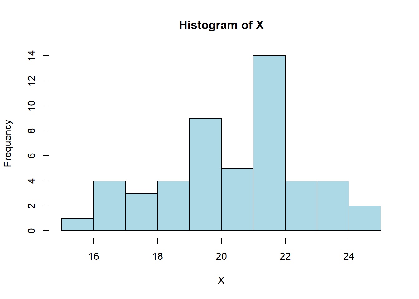
19.4 Scenario 1: Hypothesised Population Mean = 22kg
- Identify the parameter of interest: Population mean \(\large \mu\)
- Define \(\large H_O\) and \(\large H_A\)
\[\large H_O: \mu = 22\]
\[\large H_A: \mu \ne 22\]
- Define \(\large \alpha\)
\[\large \alpha = 0.05\]
- Define a significance level: \(\large \alpha = 0.05\)
- Calculate an estimate of the parameter
[1] 20.35913[1] 2.193172[1] 50- Determine test statistic, its distribution when \(\large H_O\) is correct, calculate the value of test statistic from the sample.
[1] 5.290367Distribution of the test statistic
\[\large z_{Cal} \sim Normal(mean=0, sd=1)\]
- Obtain the probability under the distribution of the test statistic (two-tailed probability)
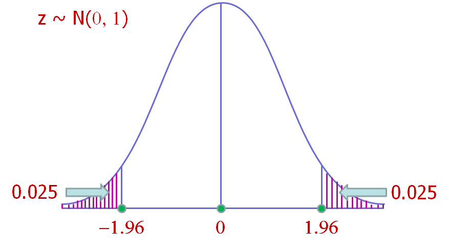
\[\large 2*pnorm(q=|z_{Cal}|, mean=0, sd=1)\]
[1] 1.220711e-07- Compare the observed probability given \(\large \alpha\) and conclude
Find the probability that \(\large z\) is less than or equal to \(\large |z_{Cal}|\) from \(\large Normal(0,1)\)
\[\large \alpha = 0.05\]
\[\large p < 0.001 \]