Section 44 Model Selection: Backward Stepwise Selection
44.1 Statistical Model
\[ \large y_{i} = \beta_0 + \beta_1 x_{1i} + \beta_2 x_{2i} + ... + \beta_p x_{pi} + \epsilon_{i} \]
\[ i = 1,...,n; \space p = \space number \space of \space predictors \]
44.2 Steps
Fit a Full model \(M_p\) which contains all \(p\) predictors.
For \(k = p,p-1,...,1\)
Consider all \(k\) models that contain all but one of the predictors in \(M_k\), for a total of \(k-1\) predictors.
Choose the best model \(M_{k-1}\) among these \(k\) models based on the smallest RSS, or equivalently, largest \(R^2\).
Select a single best model from among \(M_0, M_1, ..., M_p\) models using the criteria Adjusted \(R^2\), Mallow’s Cp, AIC or BIC.
44.4 R implementation
library(leaps)

BP <- read.csv('data/BP.csv')
# Remove NA values from all variables
BP <- na.omit(BP)
BP$DM <- as.factor(BP$DM)

# Subset the data
BP <- BP[,-1]

# Backward stepwise selection
bwd.fm <- regsubsets(SBP ~ ., data=BP,
                      nbest=1, nvmax=6, intercept=TRUE,
                      method='backward')
bwd.summary <- summary(bwd.fm)

bwd.summary
Subset selection object
Call: regsubsets.formula(SBP ~ ., data = BP, nbest = 1, nvmax = 6,
intercept = TRUE, method = "backward")
6 Variables (and intercept)
Forced in Forced out
EthnicAsian FALSE FALSE
EthnicCaucasian FALSE FALSE
Age FALSE FALSE
Income FALSE FALSE
BMI FALSE FALSE
DM2 FALSE FALSE
1 subsets of each size up to 6
Selection Algorithm: backward
EthnicAsian EthnicCaucasian Age Income BMI DM2
1 ( 1 ) " " " " " " " " "*" " "
2 ( 1 ) " " " " " " " " "*" "*"
3 ( 1 ) " " " " "*" " " "*" "*"
4 ( 1 ) " " " " "*" "*" "*" "*"
5 ( 1 ) " " "*" "*" "*" "*" "*"
6 ( 1 ) "*" "*" "*" "*" "*" "*" (Intercept) EthnicAsian EthnicCaucasian Age Income BMI DM2
-3.858060268 -0.002753277 -0.013373729 0.903319577 -0.003045831 2.348833049 4.073927322 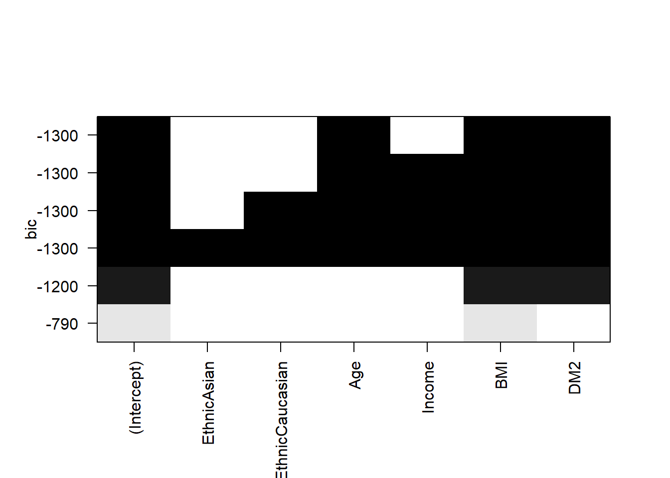
# Customised plot
par(mfrow=c(2,2))
xlab <- 'Number of X-variables'

plot(x = bwd.summary$rss,
     xlab=xlab, ylab='RSS',
     type='l', col='blue')
index <- which.min(bwd.summary$rss)
points(x = index, y = bwd.summary$rss[index],
       col='red', cex=2, pch=20)

plot(x=bwd.summary$adjr2,
     xlab=xlab, ylab='Adjusted R2',
     type='l', col='blue')
index <- which.max(bwd.summary$adjr2)
points(x = index, y = bwd.summary$adjr2[index],
       col='red', cex=2, pch=20)

plot(x=bwd.summary$cp,
     xlab=xlab, ylab='Mallow Cp',
     type='l', col='blue')
index <- which.min(bwd.summary$cp)
points(x = index, y = bwd.summary$cp[index],
       col='red', cex=2, pch=20)

plot(x=bwd.summary$bic,
     xlab=xlab, ylab='BIC',
     type='l', col='blue')
index <- which.min(bwd.summary$bic)
points(x = index, y = bwd.summary$bic[index],
       col='red', cex=2, pch=20)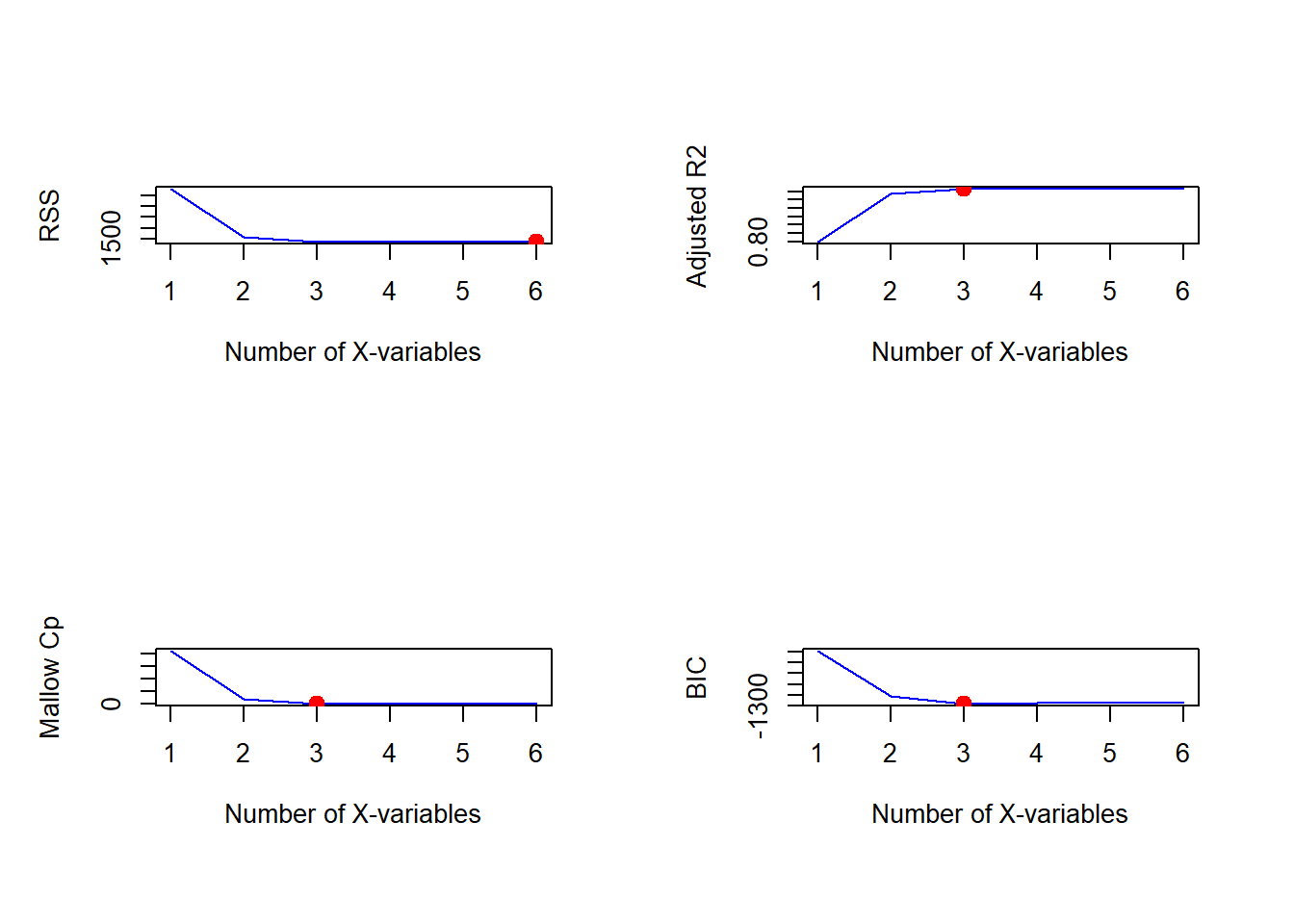
(Intercept)         Age         BMI         DM2
 -3.9018887   0.9022749   2.3487465   4.0731999
44.3 Comments
Like forward stepwise selection, this approach fits \(1 + p(p+1)/2\) models.
The backward stepwise selection also provides an efficient alternative to best subset selection.
All models within backward selection approach are nested.
However, it It is not guaranteed to find the best possible model out of all \(2^p\) models containing subsets of the \(p\) predictors.
Backward selection requires that the number of samples \(n\) is larger than the number of variables \(p\) (\(n >> p\)).