30 Fitting Machine Learning Models

• The package scikit-learn includes a comprehensive tools to conduct predictive analysis in machine learning framework

• The package is built on other packages like NumPy, SciPy and Matplotlib

• It includes modelling option for both supervised and unsupervised problems

• Methodologies include classification, regression, clustering, dimension reduction

• It also includes several supportive tools likes model selection, preprocessing, feature extraction etc.

---

30.1 Steps of model fitting

• Import specific modules of scikit-learn

• Import other relevant libraries: pandas, numpy

• Read the pandas DataFrame

• Summary information of the dataset

• Create training and testing datasets

• Exploratory analysis of the training dataset

• Build and fit the model

• Evaluate the model on the test dataset

• Explore the model performance

• Use the model to predict unseen dataset

---

30.2 Load Libraries & Read Data

Import scikit-learn

Note: We are importing modules for building a Decision Tree classifier

from sklearn.model_selection import train_test_split

from sklearn.model_selection import cross_val_score

from sklearn import metrics

from sklearn.tree import DecisionTreeClassifier, plot_tree

Import other libraries

import pandas as pd

import numpy as np

import matplotlib.pyplot as plt

Set the working directory to the data folder

Read the iris dataset as a Python object DF

DF = pd.read_csv('iris.csv')

---

30.3 Data Summary

Note: The code demonstrates only a selective summary

# Describe the data
DF.describe()

       SepalLength  SepalWidth  PetalLength  PetalWidth
count   150.000000  150.000000   150.000000  150.000000
mean      5.843333    3.057333     3.758000    1.199333
std       0.828066    0.435866     1.765298    0.762238
min       4.300000    2.000000     1.000000    0.100000
25%       5.100000    2.800000     1.600000    0.300000
50%       5.800000    3.000000     4.350000    1.300000
75%       6.400000    3.300000     5.100000    1.800000
max       7.900000    4.400000     6.900000    2.500000

# Summary by group
DF.groupby('Species').size()

Species
setosa        50
versicolor    50
virginica     50
dtype: int64

---

30.4 Train-Test Split

# Train-Test split
train, test = train_test_split(DF, test_size = 0.3, stratify = DF[['Species']], random_state = 1234)

print('Full Data: ', DF.shape)

Full Data:  (150, 5)

print('Train: ', train.shape)

Train:  (105, 5)

print('Test: ', test.shape)

Test:  (45, 5)

---

30.5 Cross-validation

We can employ a procedure called cross-validation (CV) using the training data rather than defining a train and validation split. This provides a more effective way to determine the generalisation performance when comparing models or parameters. The following implementation is depicted here:

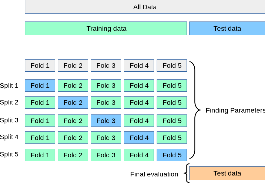
Five-fold cross-validation strategy

Image credit: scikit-learn

Import the ShuffleSplit function which allows you to define the number of folds, and the proportion of data for testing, in this case 30%.

from sklearn.model_selection import ShuffleSplit

cv = ShuffleSplit(n_splits=5, test_size=0.3, random_state=0)

Once you have defined the splits, you can pass this to the cross_val_score which is described in section on fitting the classification model with cross-validation.

---

30.6 Exploratory Data Analysis

Note: The code demonstrates only a selective exploratory data analysis; it is not comprehensive.

# Scatter plot matrix
sns.pairplot(train, hue = 'Species', palette = 'colorblind')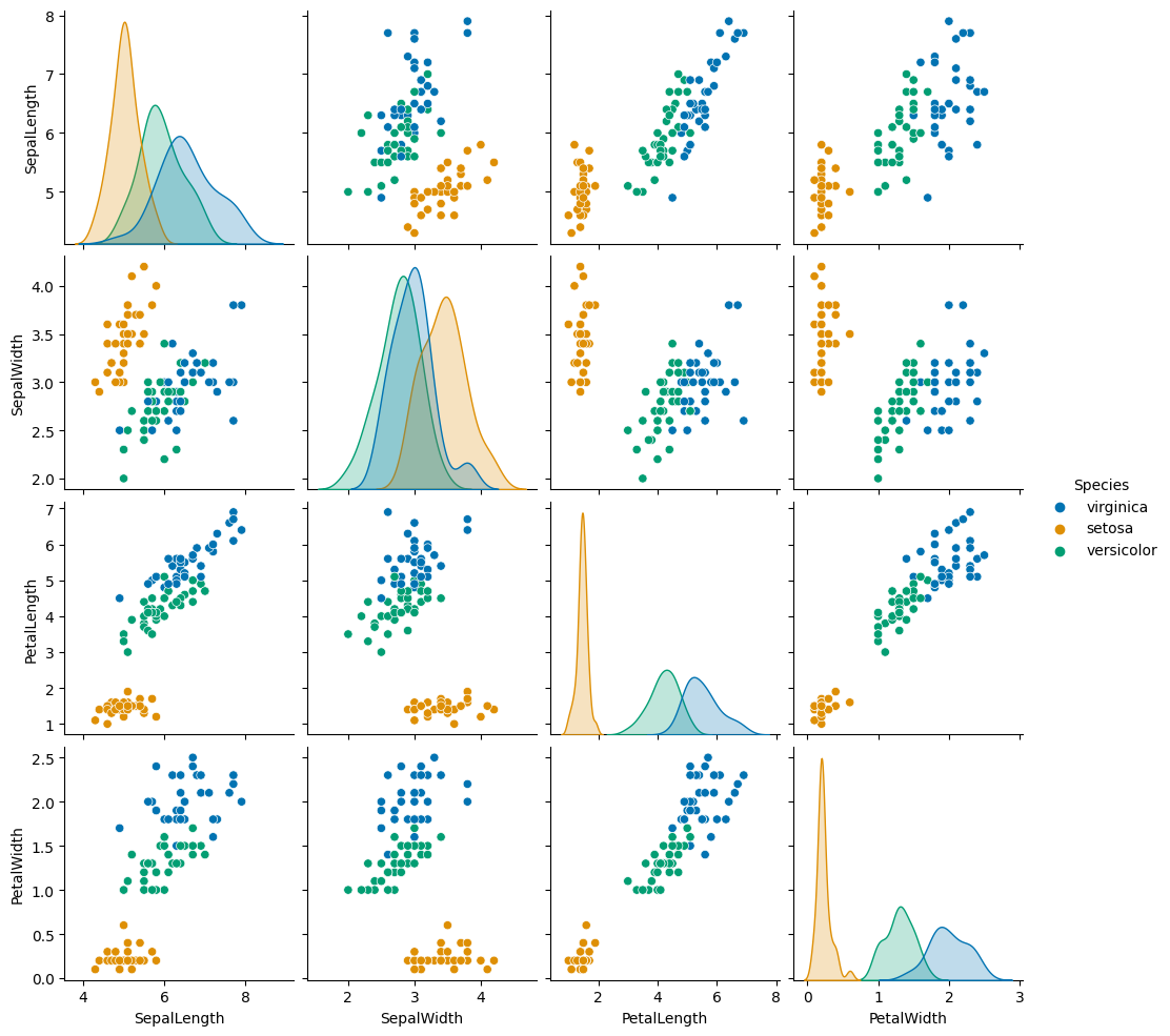

# Correlation plot
plt.clf()
corrmat = train.corr()
sns.heatmap(corrmat, annot = True, square = True);
plt.show()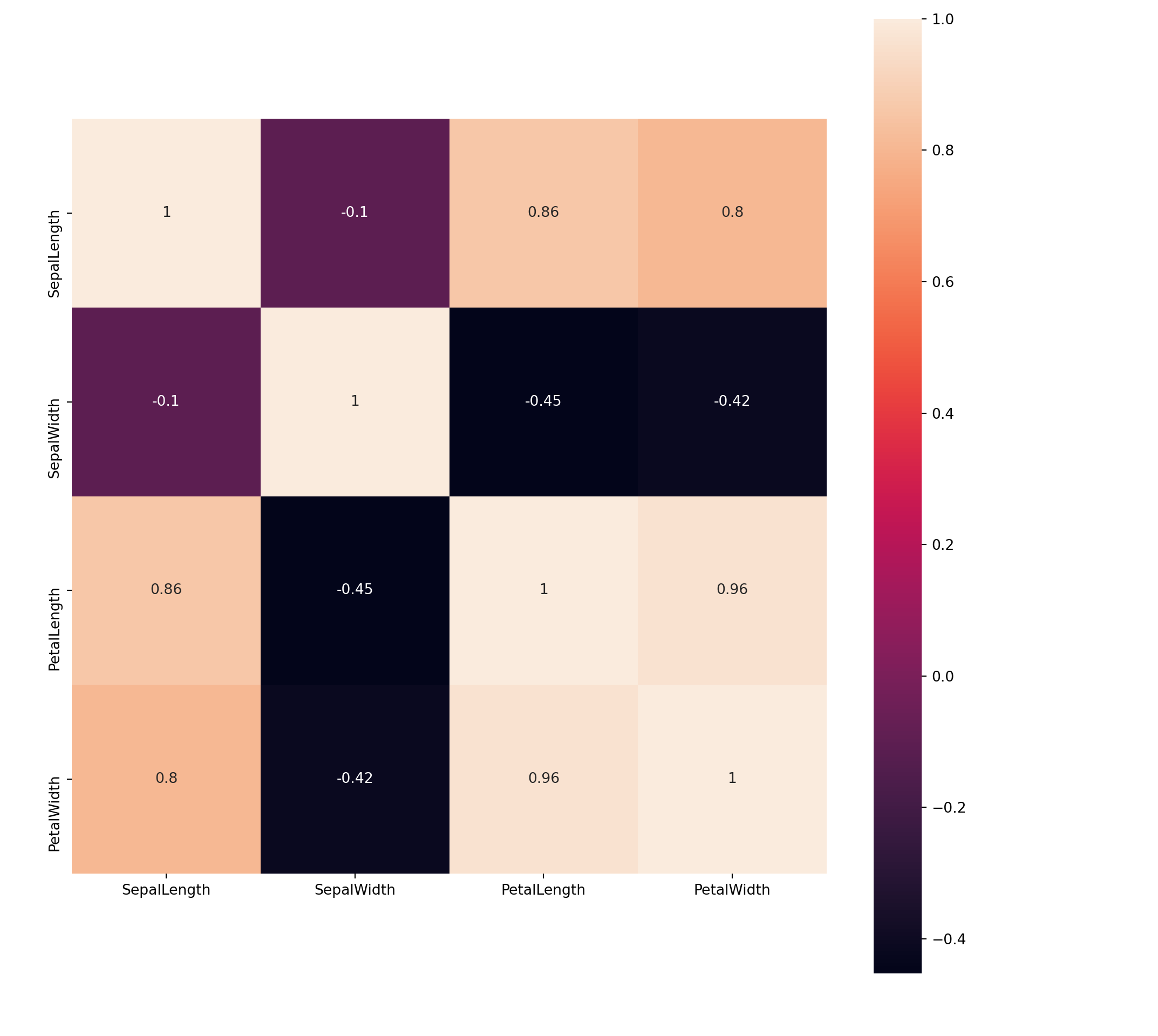

---

30.6.1 Build and fit the classification model

Here, we build a Decision Tree classifier

X_train = train.drop(['Species'], axis = 1)
y_train = train[['Species']]

X_test = test.drop(['Species'], axis = 1)
y_test = test[['Species']]

# feature names
fn = X_train.columns

# class names
cn = ['setosa', 'versicolor', 'virginica']

clf_DT = DecisionTreeClassifier(max_depth = 3, random_state = 123)

clf_DT.fit(X_train, y_train)

DecisionTreeClassifier(max_depth=3, random_state=123)

Note: Python allows all assignments in a single line

X_train, y_train, X_test, y_test = train.drop(['Species'], axis = 1), train[['Species']], test.drop(['Species'], axis = 1), test[['Species']]

---

30.6.2 Test the model on Test data

Note

test_pred provides the class names

test_prob provides the probability for each class names

test_pred = clf_DT.predict(X_test)

test_prob = clf_DT.predict_proba(X_test)

print('Test Prediction: ', test_pred.shape)

Test Prediction:  (45,)

---

30.6.3 Model Performance Metrics

print('Model Accuracy: ', f'{metrics.accuracy_score(test_pred, y_test): 0.4f}')

Model Accuracy:   0.9556

print("Precision, Recall, Confusion matrix, in training\n")

# Precision Recall scores

Precision, Recall, Confusion matrix, in training

print(metrics.classification_report(y_test, test_pred, digits = 3))

# Confusion matrix

              precision    recall  f1-score   support

      setosa      1.000     1.000     1.000        15
  versicolor      0.933     0.933     0.933        15
   virginica      0.933     0.933     0.933        15

    accuracy                          0.956        45
   macro avg      0.956     0.956     0.956        45
weighted avg      0.956     0.956     0.956        45

print(metrics.confusion_matrix(y_test, test_pred))

[[15  0  0]
 [ 0 14  1]
 [ 0  1 14]]

plt.clf()

CM = metrics.plot_confusion_matrix(clf_DT, X_test, y_test, normalize = None)
                                 
CM.ax_.set_title('Decision Tree Confusion matrix, without normalization');

# plt.show()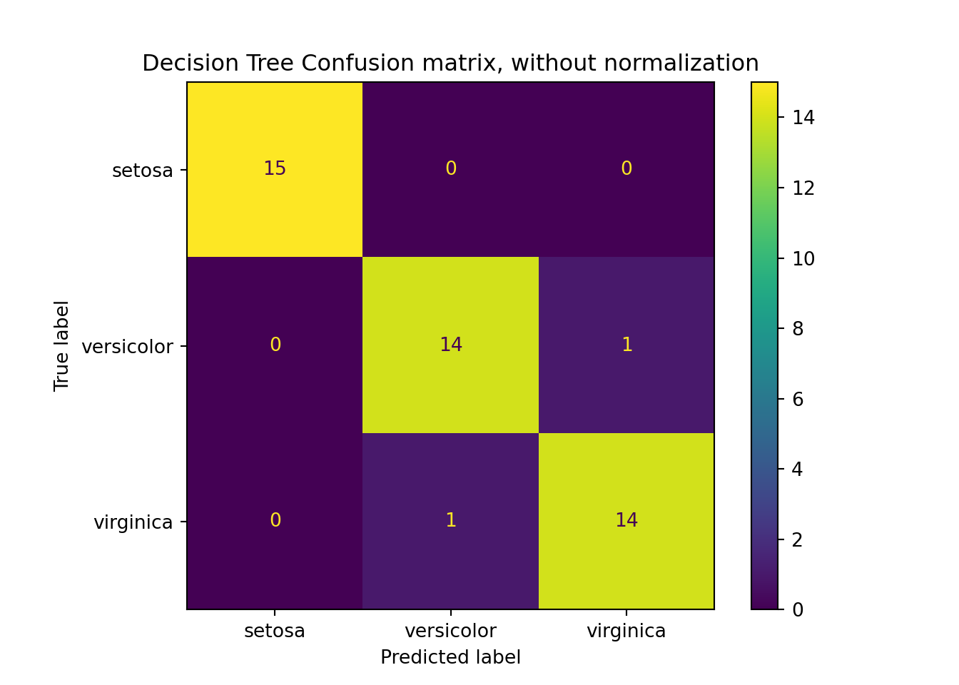

---

Fit the classification model with cross validation

To employ cross validation on our previously defined folds, simply import the cross_val_score function and append the following lines after you have fit the model.

from sklearn.model_selection import cross_val_score

scores = cross_val_score(clf_DT, x_train, y_train, cv=cv, scoring='accuracy')

This will produce 5 accuracy performance metrics per fold, which we configured to be 5.

---