6 Analysis of Paired Data: Linear Mixed Model

6.1 Research objective

To identify if the mean SBP at Week 4 decreased from the baseline value in the Treatment group

6.2 Data

We will use part data to explore this specific objective
Part data are comprised of those in the Treatment group at Week 0 and 4 for GP = 1 only

6.3 Data Summary: Plot

6.4 Data Summary: Table

Time	N	Mean	SD
0	10	146	9.10
4	10	135	7.26

6.5 Model equation

Let’s try to develop a statistical model for the given experiment.

\[y_{i4} = b_{0i} + \beta_1 \times [TIME_i = 4] + e_{i4}\]

Here:

\(y_{i4}\) = the SBP value of the i-th patient (\(i = 1, ..., 10\)) at week 4

\(b_{0i}\) = the value of SBP of the i-th patient (\(i = 1, ..., 10\)) at the baseline (week 0)

\(\beta_1\) = the difference of mean SBP at weeks 4 and 0

\(e_{i4}\) = the random error at week 4

Now, \(b_{0i}\) i.e. the value of SBP for the i-th patient at the baseline (week 0) can be modelled as:

\[b_{0i} = \beta_0 + u_{0i}\]

\(\beta_0\) = the intercept, i.e. the overall mean SBP at the baseline

\(u_{0i}\) = the effect of i-th patient (\(i = 1, ..., 10\)) at the baseline (week 0); this represents how each individual patient differs from the overall mean SBP \(\beta_0\).

Putting both models together, we have:

\[y_{i4} = (\beta_0 + u_{0i}) + \beta_1 \times [TIME_i = 4] + e_{i4}\]

Or, we can rewrite the model as:

\[y_{i4} = \beta_0 + \beta_1 \times [TIME_i = 4] + u_{0i} + e_{i4}\]

Assumptions of the above model:

\(u_{0i} \sim N(0, \sigma_P^2)\)

\(e_{i4} \sim N(0, \sigma_e^2)\)

The current scenario is a special case with two time points (baseline or week 0 and week 4) and \(TIME\) as a factor variable, \(\beta_0\) is the mean SBP at the baseline and \(\beta_1\) is the difference of mean SBP at weeks 4 and 0.

Hence, a general model framework can be presented as:

\[y_{ij} = \beta_0 + \beta_1 \times TIME_{ij} + u_{0i} + e_{ij}\]

Here:

\(y_{ij}\) = the SBP value of the i-th patient at the j-th time point

\(\beta_0\) = the intercept at the reference level of time (baseline value)

\(\beta_1\) = the effect at j-th time

\(u_{0i}\) = the effect of i-th patient associated with the intercept

\(e_{ij}\) = the random error

Assumption:

\(u_{0i} \sim N(0, \sigma_P^2)\)

\(e_{ij} \sim N(0, \sigma_e^2)\)

Note that the model is presented as a general form that can also consider more complex experimental design.

6.6 Hypothesis

\[Null \space hypothesis, H_0: \beta_1 = 0\]

\[Alternative \space hypothesis, H_1: \beta_1 \ne 0\]

6.7 Incomplete analysis: Summary

INCOMPLETE analysis of the data adjusting for the effect of patient.

We can fit the model using GLM option in SPSS with both treatment and patient as fixed effects.

We are not showing the SPSS implementation here, but note this is an INCOMPLETE model. It is shown just to demonstrate the problem with the model.

	SBP
Predictors	Estimates	SE	CI	t-statistic	p	df
(Intercept)	128.50	3.58	120.40 – 136.60	35.87	<0.001	9.00
fTime [T0]	11.00	2.16	6.11 – 15.89	5.09	0.001	9.00
ID [3]	21.00	4.83	10.07 – 31.93	4.35	0.002	9.00
ID [5]	7.00	4.83	-3.93 – 17.93	1.45	0.181	9.00
ID [6]	6.50	4.83	-4.43 – 17.43	1.35	0.211	9.00
ID [7]	3.00	4.83	-7.93 – 13.93	0.62	0.550	9.00
ID [10]	-1.00	4.83	-11.93 – 9.93	-0.21	0.841	9.00
ID [11]	-4.00	4.83	-14.93 – 6.93	-0.83	0.429	9.00
ID [12]	13.00	4.83	2.07 – 23.93	2.69	0.025	9.00
ID [17]	12.00	4.83	1.07 – 22.93	2.48	0.035	9.00
ID [20]	7.50	4.83	-3.43 – 18.43	1.55	0.155	9.00
Observations	20
R² / R² adjusted	0.885 / 0.757

The estimate (CI) for Time 4 is similar to the paired t-test based approach, hence, conceptually, we are obtaining the same estimated difference between Week 4 and baseline adjusting for the patient effect. However, note that the intercept in this model has a slightly different meaning. It is the mean SBP of the first patient in our data.

However, there are some issues with this approach.

Using Patient effect similar to the Treatment effect will use additional degrees of freedom for patients
Estimated Patient effect is not useful for practical application of the model
We cannot obtain any meaningful prediction from this model
It is possible to fit a correct model in SPSS GLM differently (using generalised least squares approach), however, we will not cover it here

6.8 Correct analysis

CORRECT analysis of the data considering the patient as a random effect. More on the random effect later.

Let’s see how we can analyse the data considering the time as a fixed effect and patient as a random effect using SPSS.

6.9 SPSS implementation

Note that for implementing linear mixed model, you have to create the long format of the data with SBP at Week 0 T0 and Week 4 T4. You can create the long format of the data and select the data only with T0 and T4 using Select Cases option. The restructured data that we created before will not work as it did not stack SBP at Week 0.

Alternatively, you can directly load the long format data for the Treatment group with two time points that we already created: SBP_GP1_Treatment_W0_W4_long.sav

Follow the steps below in SPSS to fit a linear mixed model once you load the data. We will go into the details of each step later.

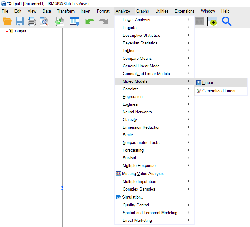
Analyze > Mixed Models > Linear

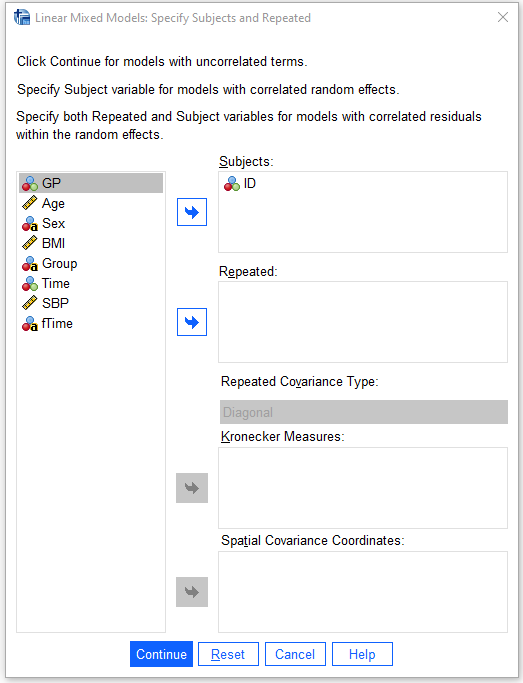
Select ID under Subjects and click Continue

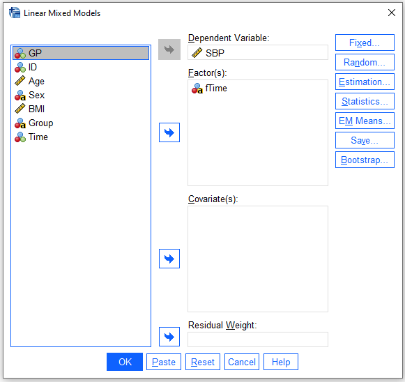
Select SBP as Dependent Variable and fTime as a Factor

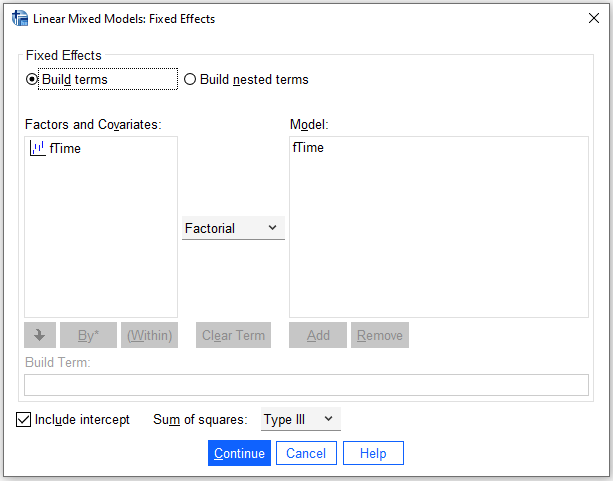
Click Fixed button, select Main effects, Add fTime to Model and click Continue

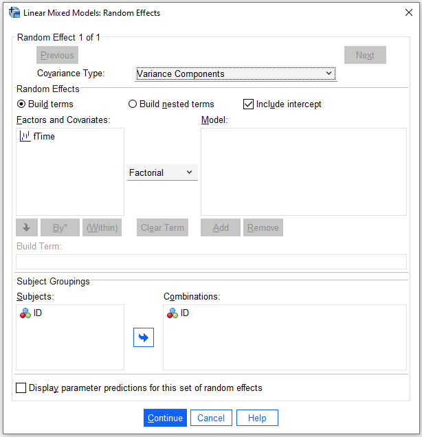
Click Random button, select Variance Components as Covariance Type, check Include Intercept, include ID to Combinations and click Continue

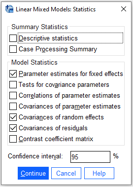
Click Statistics button, check Parameter estimates for fixed effects and Covariances of random effects and click Continue

6.10 SPSS Syntax

DATASET ACTIVATE DataSet2. 

MIXED SBP BY fTime 
  /CRITERIA = DFMETHOD(SATTERTHWAITE) CIN(95) MXITER(100) MXSTEP(10) 
   SCORING(1) SINGULAR(0.000000000001) HCONVERGE(0, ABSOLUTE) 
   LCONVERGE(0, ABSOLUTE) PCONVERGE(0.000001, ABSOLUTE) 
  /FIXED = fTime | SSTYPE(3) 
  /METHOD = REML 
  /PRINT = G R SOLUTION 
  /RANDOM = INTERCEPT | SUBJECT(ID) COVTYPE(VC).

6.11 Correct analysis: Summary

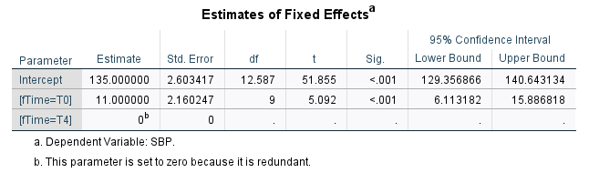
Summary of the CORRECT analysis of the data considering the patient as a random effect.

Here, we present only part of the outputs focussing on the estimated effect.

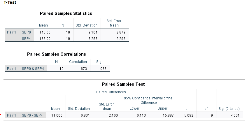
6.12 Outputs: Paired t-test

Here is the summary of outputs from the paired t-test

6.13 Explanation

Estimated effect and SE are identical for both paired t-test and linear mixed model
Note also that the t-statistic, degrees of freedom are identical