8 Terminologies

8.1 Fixed factor

For fixed factor, all possible levels of the factor are present in the study
Since all levels are included in the study, if we sample the data again, we will obtain the identical levels of the factor
For example, we may assign the variable Sex as two levels: Male and Female. If we do collect another sample, the levels of Sex in the new sample will be among these two levels.
In general, the fixed factor has few levels

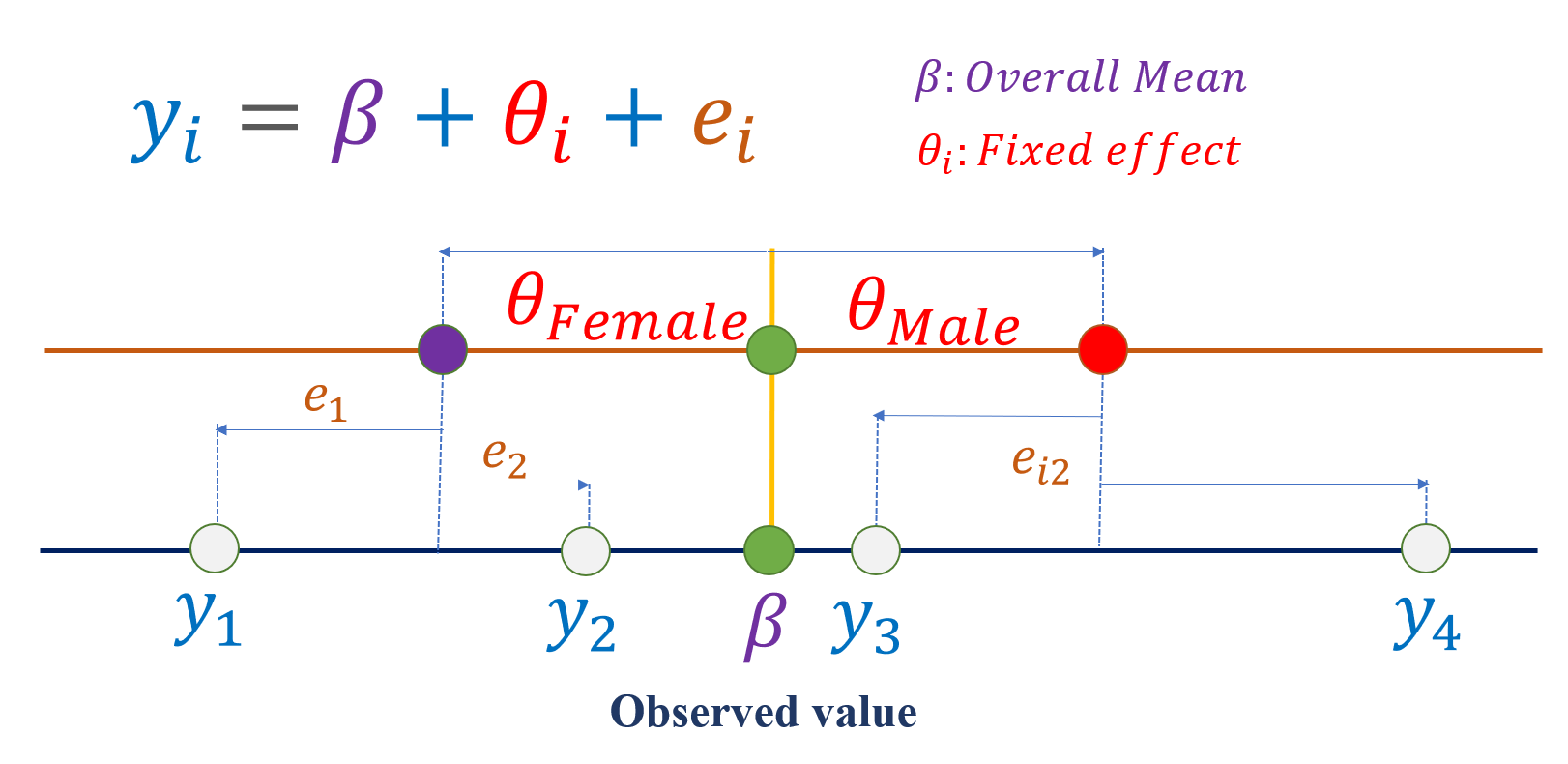
Fixed effect refers to the inference about the effect size for the levels of fixed factor
Fixed effect inference can only be made about the specific level used in the study
Fixed effect is an unknown fixed or constant quantity for the given study
Numerical variables are always considered as fixed effects

Figure: An illustration of the fixed effect and random error for the observed value of four subjects

The factor for which only a random sample of all possible levels of the factor are included in the study, i.e. the study does not include all levels of the factor
If we sample the data again, we will obtain different levels of the factor at each sampling stage
For example, we may sample patients from the population, and if we sample again, we will get a different set of patients from the population of patients.
Generally, random factor has many levels
The classification variables that identify the Level 2 and Level 3 units are considered as random factors

Random effect refers to the inference about the effect size for the levels of random factor
It usually represents random deviations from the relationships described by the fixed effects
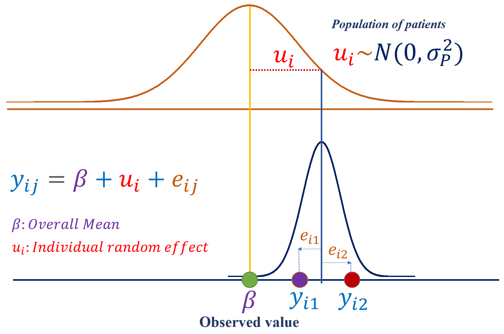
Random effect assumes the effect is randomly varying with a defined distribution, which is generally a Normal distribution
Random effect allows to make inference beyond the specific level included in the study. For example, we can generalise the inference to the population of patients, and therefore, the inference is not specific to patients included in the study
Commonly, random effects in a study are not of primary interest; or random factor is considered as a nuisance variable

Figure: An illustration of the distribution of random effect and error components for a single subject

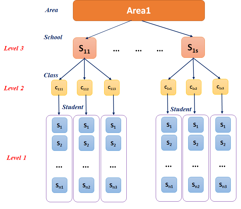
All levels of a factor (first) are measured only with a single level of another factor (second)
The first factor is then said to be nested within the levels of the second factor
The effect estimated of the nested factor on the response variable is called as nested effect

Figure: An illustration of nested factors where Students are nested within the Class, and Classes are nested within School.

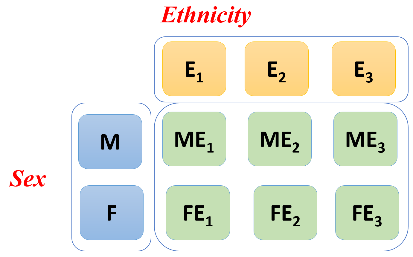
All levels of a factor (first) are measured across all levels of another factor (second)
The effects of these factors on the response variable is called crossed effects

Figure: An illustration of crossed factors where data were measured for all combination of two levels of Sex and three levels of Ethinicity.

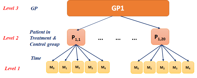
Figure: A schematic representation of the clinical data structure described above

If we wish to compare the effect of group on the SBP data at week 4 adjusting for the baseline SBP data, the model equation will be:

\[y_{i} = \beta_0 + \beta_1 \times SBP0_{i} + \beta_2 \times GROUP_{i} + \beta_3 \times (TIME_{i} = 4) + e_{i}\]

Here:

\(y_{i}\) = the SBP value of the i-th patient (\(i = 1, ..., 20\)) at Week 4

\(\beta_0\) = the intercept (fixed effect) at the reference level of group and time

\(\beta_1\) = the fixed effect of baseline SBP

\(\beta_2\) = the fixed effect of group

\(\beta_3\) = the fixed effect of time

\(e_{i}\) = the random error

Assumption:

\(e_{i} \sim N(0, \sigma_e^2)\)

If we wish to compare the effect of group on the SBP data at all time points adjusting for the baseline SBP data, the model equation will be:

\[y_{i} = \beta_0 + \beta_1 \times SBP0_{i} + \beta_2 \times GROUP_{i} + \beta_3 \times TIME_{ij} + u_{0i} + e_{ij}\]

Here:

\(y_{ij}\) = the SBP value of the i-th patient (\(i = 1, ..., 20\)) at the j-th time point (\(j = 1, 2, 3, 4\))

\(\beta_0\) = the intercept (fixed effect) at the reference level of group and time

\(\beta_1\) = the fixed effect of baseline SBP

\(\beta_2\) = the fixed effect of group

\(\beta_3\) = the fixed effect at j-th time (\(j = 2\))

\(u_{0i}\) = the random effect of i-th patient (\(i = 1, ..., 20\)) associated with the intercept

\(e_{ij}\) = the random error

Assumption:

\(u_{0i} \sim N(0, \sigma_P^2)\)

\(e_{ij} \sim N(0, \sigma_e^2)\)

Likelihood
Methods of estimation
- Restricted Maximum Likelihood (REML)
- Maximum Likelihood (ML)
Degrees of freedom
- Satterthwaite approximation
- Residual method
- Kenward-Roger approximation
Log-Likelihood convergence
Estimated Marginal (EM) Means

Complex design
Complex sampling strategies when simple random sampling within group is not applicable
Multistage sampling
Clustering of observations
Correct estimate of SE
Address missing values
Account different sources of variability
Ask complex research questions
Inference beyond the random factors included in the study