9 Multiple Time Points
9.1 Research objective
- To identify the dynamics of SBP from Week 1 to 4 in the Treatment group
9.2 Data
We will now add further complexity to our problem.
We wish to investigate the dynamics of SBP from Week 1 to 4 in the Treatment group
The data comprised of those in the Treatment group at Week 1 to 4 for GP = 1 only
Note that from now onward we will use the long-type data with baseline SBP as one of the columns
The Time column includes the time in week while the SBP column shows the corresponding SBP value
Also note that we will consider the numeric value of Time, i.e. we are interested to estimate the change in SBP (or slope) with Time.
Figure: A schematic representation of the data structure considered in this section
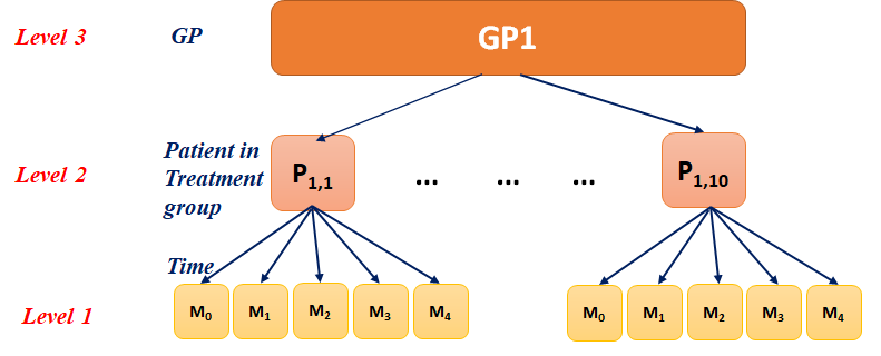
A snapshot of the data is presented here
9.3 Data Summary: Plot
9.4 Data Summary: Table
| Time | N | Mean | SD |
|---|---|---|---|
| 1 | 10 | 136.2 | 8.40 |
| 2 | 10 | 134.0 | 7.01 |
| 3 | 10 | 135.7 | 7.15 |
| 4 | 10 | 135.0 | 7.26 |
9.5 Model equation
\[y_{ij} = \beta_0 + \beta_1 \times TIME_{ij} + u_{0i} + e_{ij}\]
Here:
\(y_{ij}\) = the SBP value of the i-th patient (\(i = 1, ..., 10\)) at the j-th time point (\(j = 1, 2, 3, 4\))
\(\beta_0\) = the intercept at the reference level of time
\(\beta_1\) = the effect at j-th time (\(j = 1, 2, 3, 4\))
\(u_{0i}\) = the effect of i-th patient (\(i = 1, ..., 10\)) associated with the intercept
\(e_{ij}\) = the random error
Assumption:
\(u_{0i} \sim N(0, \sigma_P^2)\)
\(e_{ij} \sim N(0, \sigma_e^2)\)
9.6 Hypothesis
\[Null \space hypothesis, H_0: \beta_1 = 0\]
\[Alternative \space hypothesis, H_1: \beta_1 \ne 0\]
9.7 SPSS: Menu
If you are loading the long format of the data with both Treatment and Control groups, then you need to only select the Treatment group data.
Data > Select Cases > If.. > Group = "Treatment"
Only patients within Treatment group will be selected.

SPSS implementation is very similar to those presented earlier. Shown below the dialog box relevant to the inclusion of Time in the model. The random effect and rest of the model implementations are identical to those discussed in Chapter 6 ( Analysis of Paired Data: LMM ).


9.8 SPSS Syntax
MIXED SBP WITH Time
  /CRITERIA = DFMETHOD(SATTERTHWAITE) CIN(95) MXITER(100) MXSTEP(10)
    SCORING(1) SINGULAR(0.000000000001) HCONVERGE(0, ABSOLUTE)
    LCONVERGE(0, ABSOLUTE) PCONVERGE(0.000001, ABSOLUTE)
  /FIXED = Time | SSTYPE(3)
  /METHOD = REML
  /PRINT = G R SOLUTION
  /RANDOM = INTERCEPT | SUBJECT(ID) COVTYPE(VC).
9.9 Summary
The summary of model outputs from the linear mixed model considering the patient as a random effect.
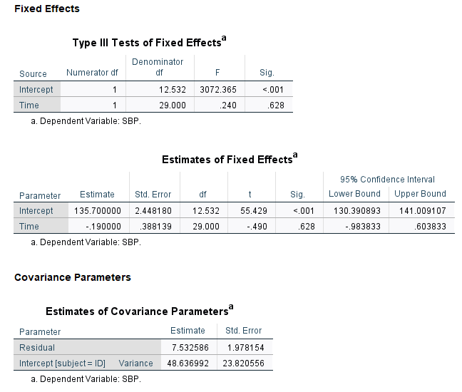
9.10 Explanation
There is no evidence in the data that the mean SBP changed from Weeks 1 to 4. However, the model does not explore our primary objective, i.e. if the overall mean SBP is different between Treatment and Control groups, and if so, the trajectory of such differences across times. We will explore this in the next section.