7 Missing Data
7.1 Research objective
- To identify if the mean SBP at Week 4 decreased from the baseline value in the Treatment group
7.2 Data
We will use part data to explore this specific objective
Part data are comprised of those in the Treatment group at Week 0 and 4 for GP = 1 only
The modelling approach we have just described is also ideal with missing observation.
The model can also borrow information at the patient’s level
Let’s imagine that five patients did not turn up on Week 4.
For example, the following five patients do not have Week 4 data: 2, 6, 7, 10, 20
The data are shown in the following table.
7.3 Data Summary: Plot
7.4 Data Summary: Table
| Time | N | Mean | SD |
|---|---|---|---|
| 0 | 10 | 146.0 | 9.10 |
| 4 | 5 | 137.4 | 8.26 |
7.5 Model equation
\[y_{ij} = \beta_0 + \beta_1 \times TIME_{ij} + u_{0i} + e_{ij}\]
Here:
\(y_{ij}\) = the SBP value of the i-th patient at the j-th time point
\(\beta_0\) = the intercept at the reference level of time (baseline value)
\(\beta_1\) = the effect at j-th time
\(u_{0i}\) = the effect of i-th patient associated with the intercept
\(e_{ij}\) = the random error
Assumption:
\(u_{0i} \sim N(0, \sigma_P^2)\)
\(e_{ij} \sim N(0, \sigma_e^2)\)
7.6 Hypothesis
\[Null \space hypothesis, H_0: \beta_1 = 0\]
\[Alternative \space hypothesis, H_1: \beta_1 \ne 0\]
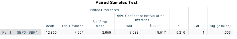
7.7 Paired t-test: SPSS Syntax
DATASET ACTIVATE DataSet1.

T-TEST PAIRS=SBP0 WITH SBP4 (PAIRED)
  /ES DISPLAY(TRUE) STANDARDIZER(SD)
  /CRITERIA=CI(.9500)
  /MISSING=ANALYSIS.
7.8 Paired t-test: Summary
The analysis of the data by paired t-test is correct, however, note that it removes all patients where paired data are not available at Week 4 resulting very low degrees of freedom for the test statistic.
7.9 LMM: SPSS Syntax
MIXED SBP BY fTime
/CRITERIA = DFMETHOD(SATTERTHWAITE) CIN(95) MXITER(100) MXSTEP(10)
SCORING(1) SINGULAR(0.000000000001) HCONVERGE(0, ABSOLUTE)
LCONVERGE(0, ABSOLUTE) PCONVERGE(0.000001, ABSOLUTE)
/FIXED = fTime | SSTYPE(3)
/METHOD = REML
/PRINT = G R SOLUTION
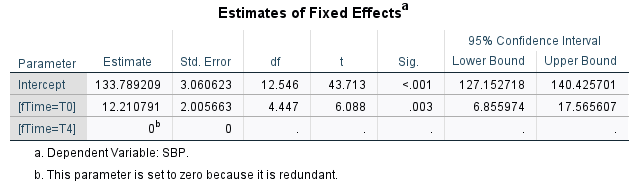
/RANDOM = INTERCEPT | SUBJECT(ID) COVTYPE(VC).7.10 Linear mixed model: Summary
The analysis of the data considering the patient as a random effect still accounts for the patients for whom the data were available at Week 0. The estimated difference between Week 4 and 0 is also different as we have more information about the baseline mean SBP than offered by a paired t-test.
Compare the estimate, SE, t-statistic, p-value for both paired t-test and linear mixed model. Although the difference is practically negligible for this small dataset with only 10 patients, in a large dataset with many patients, LMM will handle the data better than the paired t-test.
7.11 Explanation
The estimated mean SBP in the Treatment group at Week 4 decreased from the baseline value by a magnitude of about 12 mmHG.
Note that the denominator degrees of freedom may not be integer. The denominator degrees of freedom is calculated by a Satterthwaite approximation. There is other method of approximation like Kenward and Roger method. The LMM uses an approximation to estimate the denominator df.