10 Two Groups at Multiple Times

10.1 Reearch objective

• To identify the mean difference of SBP between the Treatment and Control groups and weekly changes in SBP

10.2 Data

• We will now add further complexity to our problem where we wish to include both group and time

• We wish to investigate the difference in SBP between Treatment and Control groups as well as dynamics of SBP from Weeks 1 to 4

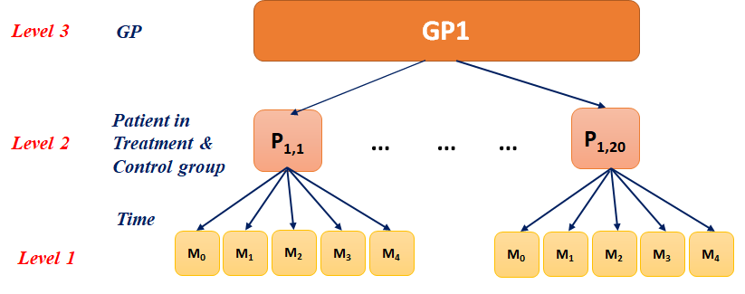
• The data comprised of those in the Treatment and Control groups at Weeks 1 to 4 for GP = 1 only

• Note that from now onward we will use long type data with baseline SBP as one of the columns

• The Time column includes the indicator of time in week while the SBP column shows the corresponding SBP value

• Also note that we will consider the integer value of Time to capture the dynamics

Figure: A schematic representation of the data structure considered in this section

A snapshot of the data is presented here

10.3 Data Summary: Plot

10.4 Data Summary: Table

Group	Time	N	Mean	SD
Control	1	10	140.4	7.75
Control	2	10	139.0	8.71
Control	3	10	138.5	7.04
Control	4	10	137.5	8.13
Treatment	1	10	136.2	8.40
Treatment	2	10	134.0	7.01
Treatment	3	10	135.7	7.15
Treatment	4	10	135.0	7.26

10.5 Model options

• Independent sample t-test between Treatment and Control groups at each time point and adjust the p-values

• Calculate the area under the curve (AUC) of the response variable against time and fit an independent sample t-test between Treatment and Control groups

• These approaches consider only part of data, therefore, may produce biased outcomes

• Additionally, there are inherent problems of model fits for unbalanced and missing data

10.6 Model equation

\[y_{ij} = \beta_0 + \beta_1 \times GROUP_{i} + \beta_2 \times TIME_{ij} + u_{0i} + e_{ij}\]

Here:

\(y_{ij}\) = the SBP value of the i-th patient (\(i = 1, ..., 20\)) at the j-th time point (\(j = 1, 2, 3, 4\))

\(\beta_0\) = the intercept at the reference level of time

\(\beta_1\) = the effect of the treatment group; \(Group = {Treatment, Control}\)

\(\beta_2\) = the effect of j-th time \(Time = {1, 2, 3, 4}\)

\(u_{0i}\) = the effect of i-th patient

\(e_{ij}\) = the random error

Assumption:

\(u_{0i} \sim N(0, \sigma_P^2)\)

\(e_{ij} \sim N(0, \sigma_e^2)\)

Model equation: extension

Model intercept consists of two components: fixed part and random part:

\[Intercept: b_{0i} = \beta_0 + u_{0i}\]

10.7 Hypothesis

Group

\[Null \space hypothesis, H_0: \beta_1 = 0\]

\[Alternative \space hypothesis, H_1: \beta_1 \ne 0\]

Time

\[Null \space hypothesis, H_0: \beta_2 = 0\]

\[Alternative \space hypothesis, H_1: \beta_2 \ne 0\]

10.8 SPSS: Menu

If you are continuing from the previous sessions, check that patients from both Treatment and Control groups are selected by opting for All cases.

Data > Select Cases > Select > All cases

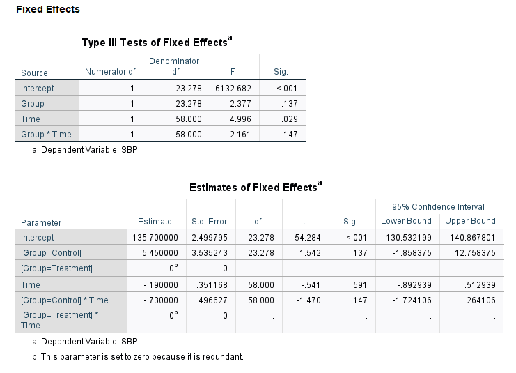
SPSS implementation is very similar to those presented earlier. Note the difference in the Factor and Covariates and how we can include the Main Effects and Interaction Terms in the Fixed Effects dialog box. The random effect and rest of the model implementations are identical to those discussed in Chapter 6 ( Analysis of Paired Data: LMM ).

10.9 SPSS Syntax

MIXED SBP BY Group WITH Time 
  /CRITERIA = DFMETHOD(SATTERTHWAITE) CIN(95) MXITER(100) MXSTEP(10) 
   SCORING(1) SINGULAR(0.000000000001) HCONVERGE(0, ABSOLUTE) 
   LCONVERGE(0, ABSOLUTE) PCONVERGE(0.000001, ABSOLUTE) 
  /FIXED = Group Time Group*Time | SSTYPE(3) 
  /METHOD = REML 
  /PRINT = G R SOLUTION 
  /RANDOM = INTERCEPT | SUBJECT(ID) COVTYPE(VC).

10.10 Summary

The summary of model outputs from the linear mixed model considering the patient as a random effect.

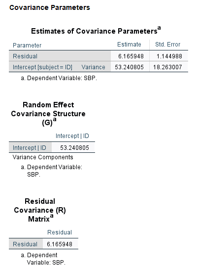
10.11 Estimates of variance

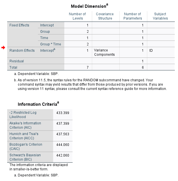
10.12 Model performance

Several statistics can be used to check the performance of the model.

10.13 Intraclass correlation (ICC)

The intraclass correlation is estimated as between patient variability to the total variability.

\[ICC = \frac{\sigma_P^2}{\sigma_P^2 + \sigma_e^2}\]

We can calcualate the ICC using the estimates of \(\sigma^2_P\) and \(\sigma^2_e\) as:

\[ICC = \frac{53.2408}{53.2408 + 6.1659} = 0.8962\]

10.14 Explanation

This model is still incomplete since we have not explored several other predictors measured at the baseline that may influence the SBP at subsequent time points. We will check the approaches to the model selection in the next section and obtain the estimated mean difference between Treatment and Control groups after adjusting for other predictor variables.