Section 34 ggplot2 `scale`

34.1 `scale`

All functions with prefix scale_ control how a plot maps data values to the visual values of an aesthetic. To change the ggplot2 default mapping, you need to add a custom scale.

Override the default scales to tweak details like the axis labels or legend keys, or to use a completely different translation from data to aesthetic. labs() and lims() are convenient helpers for the most common adjustments to the labels and limits.

Find more details here: http://ggplot2.tidyverse.org/reference/

34.2 aesthetics

aesthetics	Description
`colour`	Color of lines and points
`fill`	Color of area fills (e.g. bar graph)
`linetype`	Solid/dashed/dotted lines
`shape`	Shape of points
`size`	Size of points
`alpha`	Opacity/transparency
`x`	X-axis
`y`	Y-axis

34.3 General purpose scale

type	Description
`manual`	Map discrete values to manually-specified values (e.g., colors, point shapes, line types)
`discrete`	Map discrete values to visual values (e.g., colors, point shapes, line types, point sizes)
`continuous`	Map continuous values to visual values (e.g., alpha, colors, point sizes)
`identity`	Use data values as visual values

There are other scale types that control date, time, colour, scale of axes, shape and area. Check the ggplot2 website for further details.

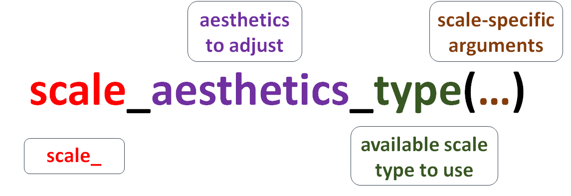
34.4 scale-specific arguments

Arguments corresponding to a type of scale
Common arguments are: values, limits, name, labels, palette

34.5 Default boxplot

g <- ggplot(data=iris, 
            mapping=aes(x=Species, y=Sepal.Length, fill=Species))
g <- g + geom_boxplot()
g <- g + labs(title='Boxplot of iris data',
              subtitle = 'Based on iris data',
              x='Species',
              y='Sepal Length (cm)')
g <- g + theme_bw()
g

34.6 Remove legends using `scale_`

# Option 3: Remove legend specifying the scale
g + scale_fill_discrete(guide=FALSE)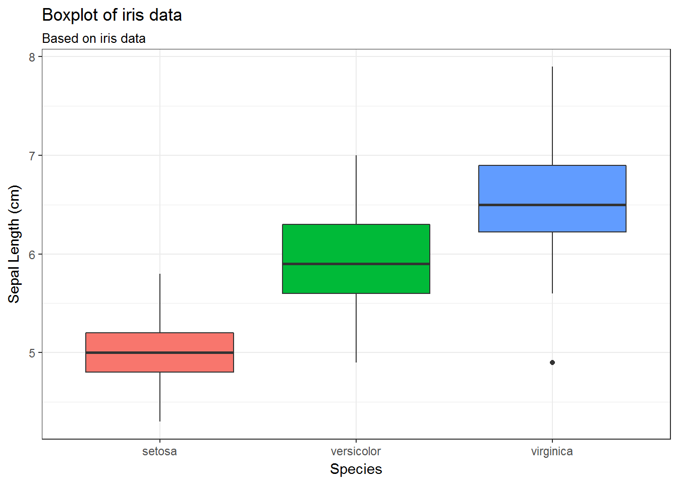

34.7 Modify legend titles and labels

g + scale_fill_discrete(name='Iris Species')

g + scale_fill_discrete(name='Iris Species',
                         breaks=c('setosa', 'versicolor', 'virginica'),
                         labels=c('Setosa', 'Versicolor', 'Virginica'))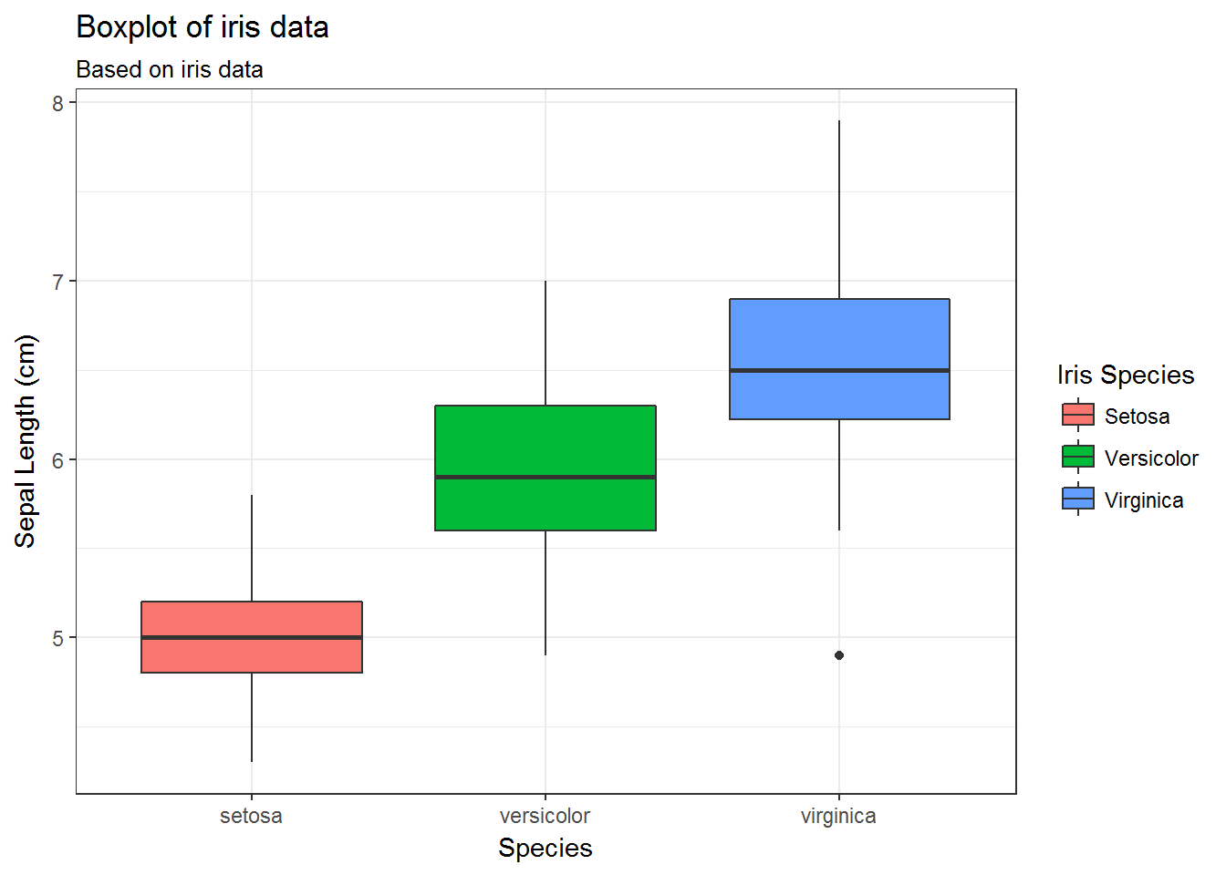

34.8 `scale_fill_manual`

g <- ggplot(data=iris, 
            mapping=aes(x=Species, y=Sepal.Length, fill=Species))
g <- g + geom_boxplot()
g <- g + stat_summary(fun.y=mean, geom='point', shape=16, size=4, colour='yellow')
g + scale_fill_manual(values=c('blue', 'pink', 'green'), 
                      name='Iris Species',
                      breaks=c('setosa', 'versicolor', 'virginica'),
                      labels=c('Setosa', 'Versicolor', 'Virginica'))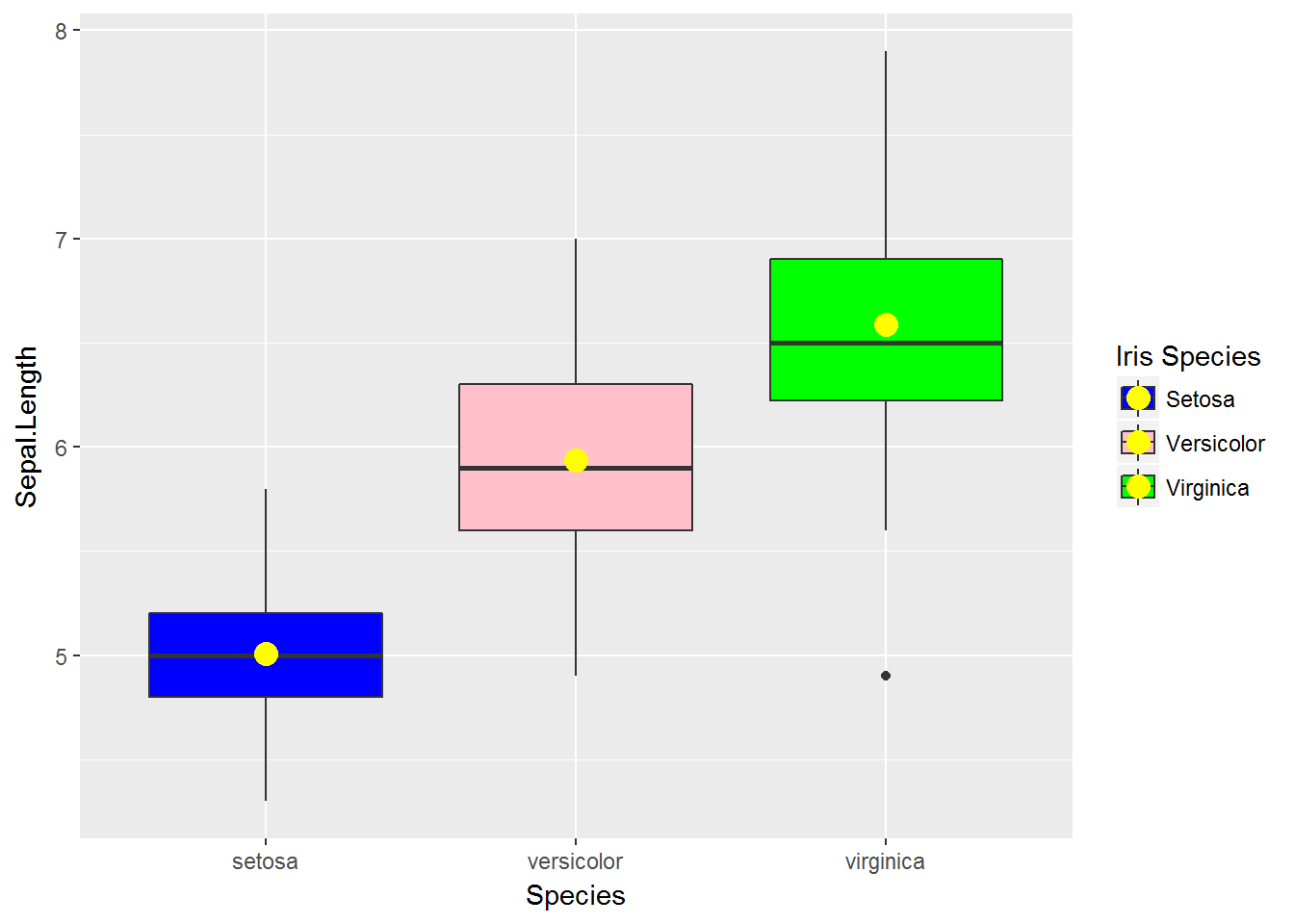

34.9 Change both x-axis and legend labels

g + scale_fill_manual(values=c('blue', 'pink', 'green'), 
                      name='Iris Species',
                      breaks=c('setosa', 'versicolor', 'virginica'),
                      labels=c('Setosa', 'Versicolor', 'Virginica')) +
    scale_x_discrete(breaks=c('setosa', 'versicolor', 'virginica'),
                     labels=c(c('Setosa', 'Versicolor', 'Virginica')))

34.10 Change the data.frame

An alternative (and easier) way to show the appropriate labels of a factor in the ggplot2 outputs, first change the labels of the factor in the data.frame, and then call ggplot2 functions.

mod.iris <- iris
mod.iris$Species <- factor(mod.iris$Species,
                   levels = c('setosa', 'versicolor', 'virginica'),
                   labels = c('Setosa', 'Versicolor', 'Virginica'))

g <- ggplot(data=mod.iris, 
            mapping=aes(x=Species, y=Sepal.Length, fill=Species))
g <- g + geom_boxplot()
g <- g + labs(title='Boxplot of iris data',
              subtitle = 'Based on iris data',
              x='Species',
              y='Sepal Length (cm)')
g <- g + theme_bw()
g

34.11 Exercise

Generate the following data.

set.seed(12345)

x <- rnorm(n = 10, mean=10, sd=2)
y1 <- 2*x + rnorm(n = 10, mean=0, sd=1)
y2 <- 4 + 2*x + rnorm(n = 10, mean=0, sd=1)
Gr <- rep(c('G1','G2'), each = 10)
DF <- data.frame(X=x, Y=c(y1,y2), ID=LETTERS[1:20], Gr=Gr)

Create the following scatter plot along with the fitted line. Change the colour of points as red and blue for Gr1 and Gr2, respectively.