Section 20 One Numeric: geom_qq
The function geom_qq produces the QQ plot of a numeric data.
20.1 Example 1:
data(iris)
# QQ plot
g <- ggplot(data=iris, mapping=aes(sample=Sepal.Length))
g <- g + geom_qq(distribution = stats::qnorm)
g
# QQ plot with QQ line
y <- iris$Sepal.Length
qy <- quantile(y, probs=c(0.25, 0.75), na.rm=TRUE)
qx <- qnorm(p=c(0.25, 0.75))
slope <- unname(diff(qy)/diff(qx))
int <- unname(qy[1] - slope*qx[1])

g <- ggplot(data=iris, mapping=aes(sample=Sepal.Length))
g <- g + geom_qq(distribution = stats::qnorm)
g <- g + geom_abline(slope=slope, intercept=int)
g
# With additional arguments
g <- ggplot(data=iris, mapping=aes(sample=Sepal.Length))
g <- g + geom_qq(distribution = stats::qnorm, col='blue')
g <- g + geom_abline(slope=slope, intercept=int, colour='red', linetype=2, size=1.25)
g <- g + labs(title='QQ plot of Sepal Length',
              subtitle='Based on Iris data',
              x='Theoretical Quantile',
              y='Sepal Length (cm)')
g + theme_bw()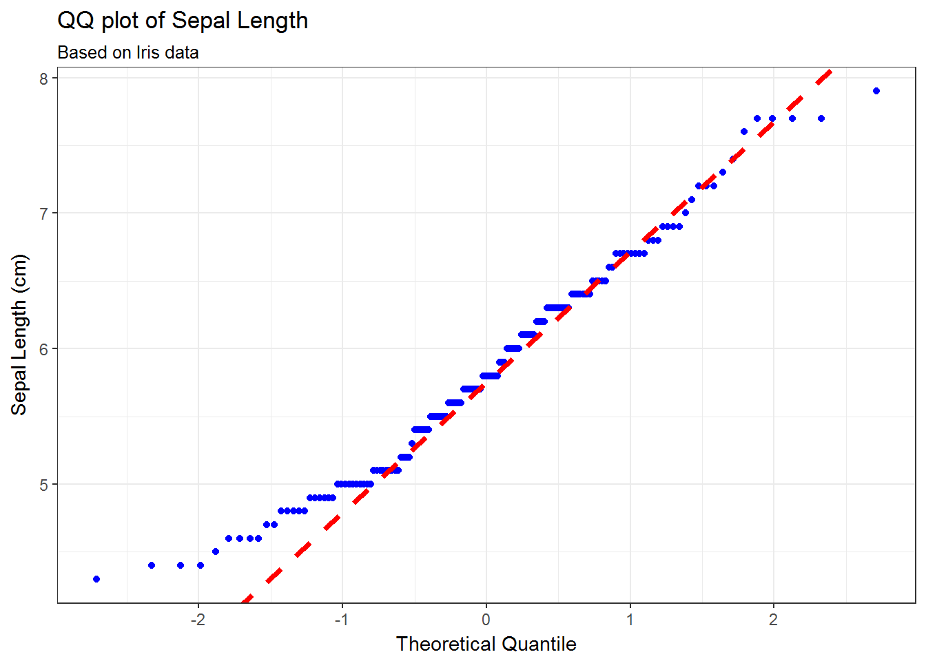
20.2 Example 2:
data(warpbreaks)
Draw a QQ plot of the variable
breaksDiscuss the QQ plot
Transform the data using log-transformation and redraw the QQ plot