Section 19 Single Continuous Variable: Density & Rug plot

19.1 Density plot

• A Density Plot visualises the distribution of data over a continuous interval.
• It is a variation of a Histogram that uses kernel smoothing to plot values, allowing for smoother distributions by smoothing out the noise.
• Density plot along with Rug plot adds additional information for the sample observations.
• Rug plot is generally used when the sample size is smaller.

19.2 package base

data(iris)

hist(x=iris$Sepal.Length, breaks=15, 
     xlim=c(4,8), freq=FALSE,
     main='Histogram of Sepal Length',
     xlab='Sepal Length (cm)',
     ylab='Density',
     axes=TRUE,
     col='orange',
     lty=1, border='purple')

lines(density(iris$Sepal.Length), col = 'red', lwd = 2, lty = 1)

rug(jitter(x=iris$Sepal.Length, amount = 0.01), side = 1, col = 'red')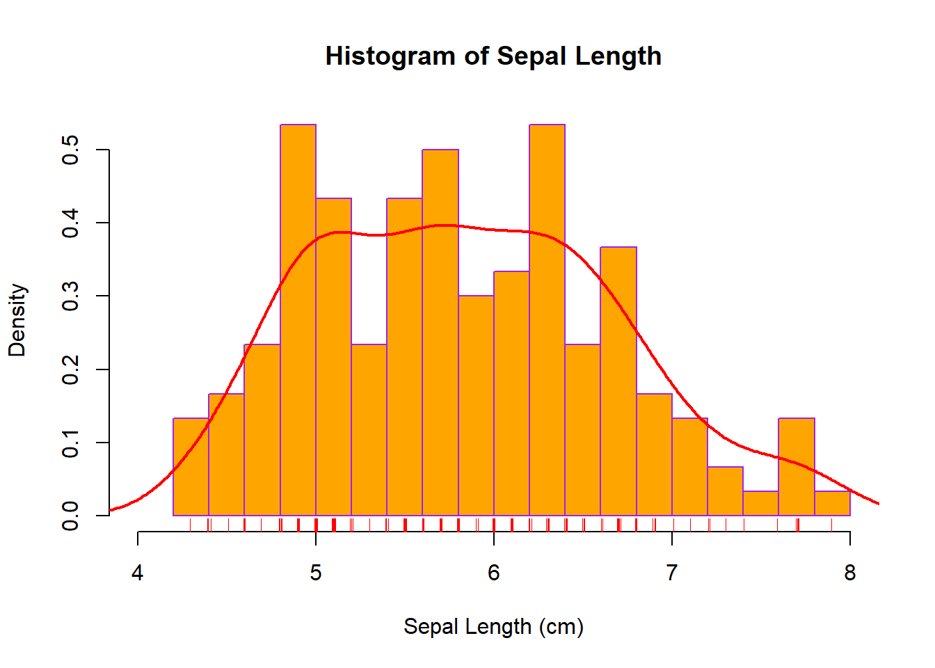

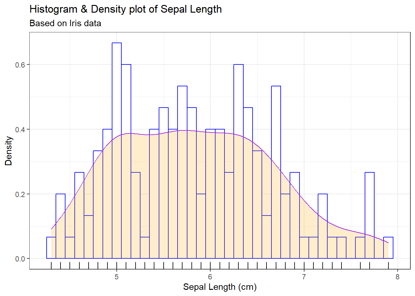
19.3 package ggplot2

g <- ggplot(data=iris, mapping=aes(Sepal.Length))
g <- g + geom_histogram(mapping=aes(y=..density..),
                        binwidth=0.10, fill='white', colour='blue')
g <- g + geom_density(alpha=0.2, fill='orange', colour='purple')
g <- g + labs(title='Histogram & Density plot of Sepal Length',
              subtitle='Based on Iris data',
              x='Sepal Length (cm)',
              y='Density')
g <- g + geom_rug()
g + theme_bw()