Section 57 Standard Normal Distribution

• The Normal distribution is the most useful and frequently occurring distribution for continuous data.

• Of particular interest is the standard normal, \(N(0,1)\), distribution, often denoted by \(z\).

• We can easily derive its shape, or density function.

    z=seq( -4, +4, .01)
    density=dnorm(z, mean=0, sd=1)
    plot(z, density, type="l")

    # curve(dnorm(x,mean=0,sd=1),from=-4,to=+4,col="green") 

For the standard normal distribution we might denote these by: \(z_{0.25}\), \(z_{0.50}\) and \(z_{0.75}\).

\[\large P(z < z_{0.25}) = 0.25\]

\[\large P(z < z_{0.50}) = 0.50\]

\[\large P(z < z_{0.75}) = 0.75\]

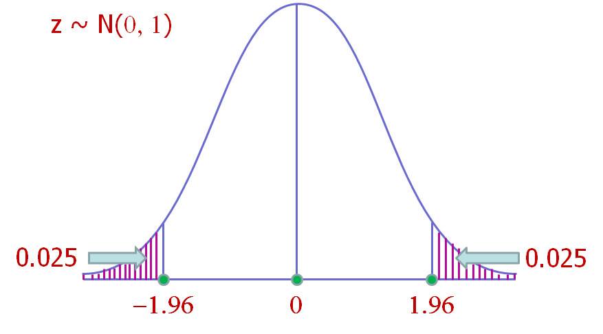
• These can be generalized to quantiles, \(z_{0.025}\) and \(z_{0.005}\)

• 2.5% quantiles of Standard Normal distribution:

\[\large P(z < z_{0.025}) = 0.025\]

• 0.5% quantiles of Standard Normal distribution:

\[\large P(z < z_{0.005}) = 0.005\]