Section 21 Single Continuous Variable: Q-Q Plot

21.1 Q-Q plot

• Q-Q (quantile-quantile) plot is a probability plot, which is a graphical method for comparing two probability distributions by plotting their quantiles against each other.
• A common use to compare the data from the observed distribution against the expected theoretical distribution.

21.2 package base

data(iris)

qqnorm(y=iris$Sepal.Length, 
       main='Normal QQ of Sepal Length',
       xlab='Theoretical Quantiles',
       ylab='Sepal Length (cm)',
       col='blue')
qqline(y=iris$Sepal.Length, lty=1, lwd=2, col='red')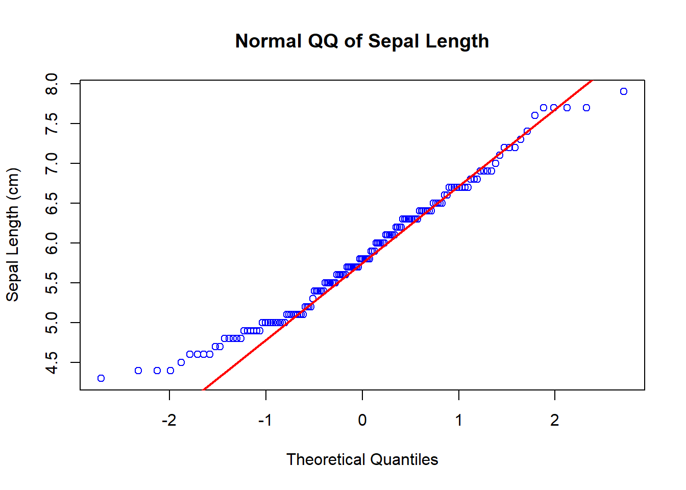

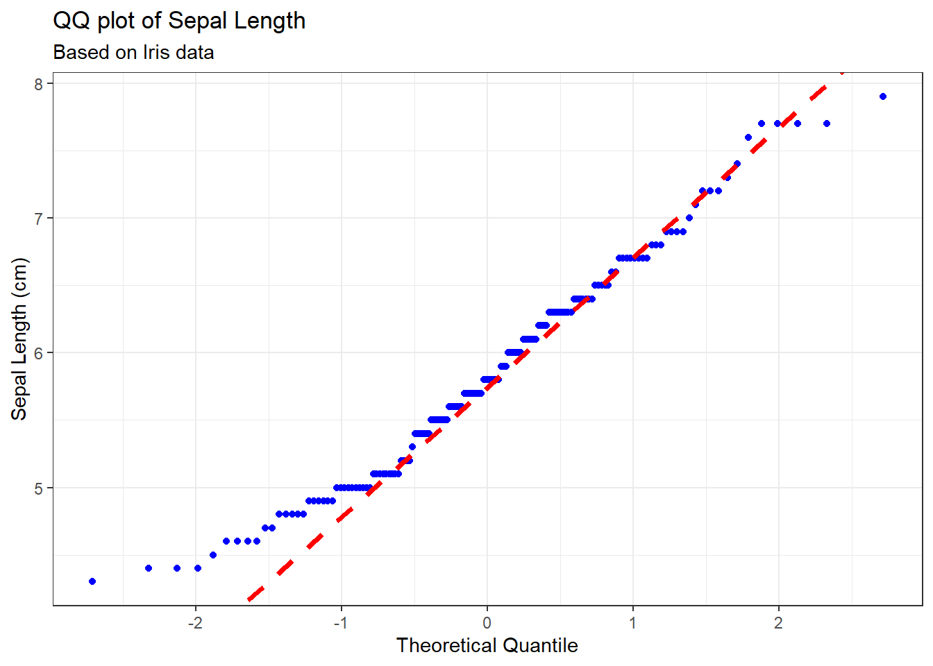
21.3 package ggplot2

# QQ plot with QQ line
y <- iris$Sepal.Length
qy <- quantile(y, probs=c(0.25, 0.75), na.rm=TRUE)
qx <- qnorm(p=c(0.25, 0.75))
slope <- unname(diff(qy)/diff(qx))
int <- unname(qy[1] - slope*qx[1])

g <- ggplot(data=iris, mapping=aes(sample=Sepal.Length))
g <- g + geom_qq(distribution = stats::qnorm, col='blue')
g <- g + geom_abline(slope=slope, intercept=int, colour='red', linetype=2, size=1.25)
g <- g + labs(title='QQ plot of Sepal Length',
              subtitle='Based on Iris data',
              x='Theoretical Quantile',
              y='Sepal Length (cm)')
g + theme_bw()